Frequency Wins: How GPT-2's Factual Retrieval Circuit Amplifies Training Bias Over Contextual Correction
Paper 1 of the Frequency Prior Trilogy. Model: GPT-2 Small (124M parameters, 12 layers, 12 heads, 768-d residual stream). Platform: TransformerLens — all results from real-model inference.
I. The Hook
We tested GPT-2 Small on a simple task: given a series of worked examples in the format "The capital of France is Paris. The capital of Japan is Tokyo...," predict the capital of a target country. The expected result was monotonic improvement — more examples, better performance. What we found instead: one example jumps accuracy from 0% to 79%. Every additional example degrades it. At five examples, accuracy has fallen to 55%. The model gets worse the more you teach it.
That behavioral result is surprising. The mechanistic result is stranger. Using activation patching and logit lens analysis, I traced the failure layer by layer through GPT-2's twelve-layer network. For countries where the model consistently gives the wrong answer — India predicting Mumbai instead of New Delhi, Australia predicting Sydney instead of Canberra — the factual signal is present and winning through layer eight of twelve. New Delhi outranks Mumbai in the residual stream at every layer from L1 through L8. Then at layer nine, Mumbai jumps from rank 235 to rank 3 in a single forward pass, overwriting a correct intermediate representation with a high-frequency alternative. The model does not lack the knowledge. It retrieves the right answer and then discards it.
Four findings, stated upfront:
One. In-context learning for factual retrieval has an optimal dosage — one example — not a monotonic benefit. Additional examples activate competing city-association pathways via the same retrieval circuit, and training-data frequency determines which association wins.
Two. For a subset of countries, the frequency-based error is not correctable by context in GPT-2 Small. The logit lens reveals two distinct failure modes: countries where the capital leads at layer 9 and gets overwritten by late-layer processing (Australia, Canada), and countries where the frequency bias is already dominant at layer 9 from the first example (India, Switzerland, South Africa). This context-immunity is itself scale-dependent and dissolves entirely by 1.5B parameters.
Three. The entropy-accuracy divergence between one and three examples means standard uncertainty monitoring would miss this failure mode entirely. The model becomes confidently wrong while appearing equally uncertain.
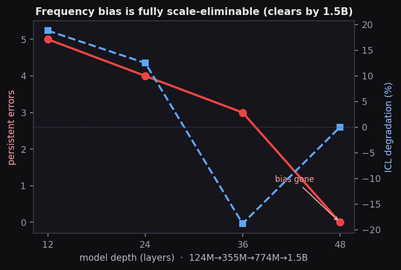
Four. Over-conditioning is a capacity-relative phenomenon, not a fixed architectural defect. Sweeping the full GPT-2 family (124M → 355M → 774M → 1.5B) reveals three regimes: over-conditioning that degrades accuracy (Small, Medium); a constructive regime where examples help (Large); and saturation where accuracy is flat and near-perfect (XL). Persistent error count falls monotonically: 5 → 4 → 3 → 0.
II. Background
The assumption baked into most work on in-context learning is that more examples help. The original GPT-3 paper (Brown et al., 2020) demonstrated monotonic improvement as shot count increased, and the field largely inherited that framing. Recent work has complicated this picture without explaining it mechanistically. Liu et al. (2023) showed information position affects retrieval; work on over-prompting in GPT-4o and LLaMA-class systems has documented accuracy degradation beyond a threshold. None provided a mechanistic account: which components change as examples accumulate, and why does additional context hurt?
That is the gap this work addresses, using a deliberately small and transparent model. GPT-2 Small has 124M parameters, 12 transformer layers, 12 attention heads per layer, and a 768-dimensional residual stream. TransformerLens (Nanda & Bloom, 2022) provides clean APIs for activation patching, residual stream inspection, and attention weight extraction. The trade-off is explicit: this is a study of mechanisms, not capabilities. Specific numbers are properties of GPT-2 Small and should not be extrapolated without further investigation, which we undertake across the full GPT-2 family in Section IX.
III. Methodology
An honest account of the simulation discovery. The early phase of this project was conducted on an iPad using Pythonista. The transformer library in use had a demo mode that activated silently when PyTorch was unavailable — returning plausible-looking but entirely fabricated outputs. The discovery came from an entropy check: real GPT-2 Small produces full-vocabulary entropy between 3.5 and 11 bits. Every result from the early runs showed entropy capped at 2.16 bits. All prior results were retired. Everything reported here comes from verified real-model runs via TransformerLens on Google Colab.
A hard entropy gate (threshold: 1.5 bits) now gates every experimental run before any result is recorded. A secondary check: all token measurements were verified against GPT-2's BPE vocabulary via model.to_str_tokens(). An earlier script version used incorrect first-tokens for three cities (Johannesburg: " Jo" instead of " Johannes", Zurich: " Z" instead of " Zurich", Canberra: " Can" instead of " Canberra"), producing anomalous results caught and corrected before final analysis.
Experimental setup. Prompt structure: "The capital of France is Paris. The capital of Japan is Tokyo. [...] The capital of {target} is". ICL examples added in order: France, Japan, Germany, Italy, Spain. Test set: 25 countries. The logit lens projects the residual stream through the unembedding matrix at all 13 checkpoints (embedding + 12 transformer blocks). Activation patching uses a clean prompt (one-shot, correct country) vs. corrupted prompt (country replaced with "Dead"), patching each head and MLP layer individually across 7 countries.
IV. The Inverted Gradient
The accuracy curve
| n examples | Countries tested | Accuracy | Mean confidence | Entropy (bits) |
|---|---|---|---|---|
| 0 | 25 | 0.0% | 0.057 | 8.59 |
| 1 | 24 | 79.2% | 0.526 | 3.83 |
| 2 | 23 | 73.9% | 0.505 | 3.64 |
| 3 | 22 | 68.2% | 0.500 | 3.68 |
| 5 | 20 | 55.0% | 0.371 | 4.90 |
The jump from zero-shot to one-shot is dramatic and statistically robust: McNemar's χ² = 17.05, p < 0.0001, with 19 countries improving and none degrading. Every additional example then degrades performance monotonically — a 24-point drop from the one-shot peak to five-shot.
The calibration story: the model becomes confidently wrong
Three calibration observations tell the fuller story.
Weakening evidence. The McNemar chi-squared statistic decreases monotonically with n: 17.1 at n=1, 15.1 at n=2, 13.1 at n=3, 9.1 at n=5.
Calibration compression. At n=1, the confidence gap between correct and incorrect predictions is +0.204. At n=2 and n=3, this compresses to +0.127 and +0.130 while accuracy falls. The model is becoming more confident on wrong answers.
The entropy-accuracy divergence. Between n=1 and n=3, full-vocabulary entropy decreases slightly (3.83 → 3.64 → 3.68 bits) while accuracy falls 11 points. A monitoring system watching entropy would see nothing unusual — the failure is invisible to standard diagnostics.
V. The Famous-City Errors
Five countries that never resolve
Across all shot counts from one to five, five countries produce the same wrong answer every time:
| Country | Capital | Model predicts | Confidence at n=1 |
|---|---|---|---|
| India | New Delhi | Mumbai | 43.1% |
| Australia | Canberra | Sydney | 35.5% |
| Canada | Ottawa | Toronto | 26.6% |
| Switzerland | Bern | Zurich | 28.8% |
| South Africa | Pretoria | Johannesburg | 48.3% |
Every wrong answer is the most globally prominent city in that country rather than the political capital. South Africa→Johannesburg strengthens with examples: 48.3% at n=1, 76.9% at n=3.
Emergent errors
Four additional countries produce correct answers at n=1 but flip as examples accumulate: Turkey (Ankara → Istanbul at n=2), China (Beijing → Shanghai at n=3), Mexico (Mexico City → "San" at n=5), Belgium (Brussels → Barcelona at n=5).
Belgium→Barcelona is particularly instructive. Spain is one of the five example countries. The model is not confusing Brussels with another Belgian city — it is bleeding the Spanish city-name pattern into a semantically adjacent slot. Cross-country association contamination.
Grounding the frequency claim in training data
We streamed 50,000 documents from OpenWebText and counted whole-word occurrences of each city:
| Country | Capital (count) | Famous city (count) | Ratio | Error? |
|---|---|---|---|---|
| India | New Delhi (403) | Mumbai (411) | 1.02× | ✓ |
| Australia | Canberra (171) | Sydney (1428) | 8.35× | ✓ |
| Canada | Ottawa (934) | Toronto (2834) | 3.03× | ✓ |
| Switzerland | Bern (58) | Zurich (107) | 1.85× | ✓ |
| South Africa | Pretoria (47) | Johannesburg (117) | 2.49× | ✓ |
Control countries run the other way: Japan (Tokyo 870 vs. Osaka 79, 0.09×), Germany (Berlin 1031 vs. Munich 362, 0.35×). The capital dominates the corpus and the model gets them right.
The India caveat. India's raw ratio barely exceeds one (1.02×), and its co-occurrence ratio inverts: near the word "India," New Delhi appears more often than Mumbai (152 vs. 100, 0.66×). The frequency advantage is global, not local. MLP0's frequency prior tracks global token salience, not country-conditioned co-occurrence.
Brazil: frequency skew without error. São Paulo outnumbers Brasília 5.17× — larger than any error country — yet Brazil is not an error country. Brasília ranks first in the retrieval format. This sharpens the claim: corpus-frequency skew is necessary but not sufficient. Frequency tips a balance that must already exist; it does not create one from nothing.
VI. Where the Failure Happens: the Logit Lens
India: the model knows the right answer through Layer 8
| Layer | Delhi rank | Mumbai rank | Winner | Logit diff |
|---|---|---|---|---|
| L1 | 2,064 | 27,287 | ✓ Delhi | +5.43 |
| L4 | 3,863 | 7,207 | ✓ Delhi | +1.33 |
| L7 | 390 | 2,576 | ✓ Delhi | +3.21 |
| L8 | 49 | 235 | ✓ Delhi | +2.40 |
| L9 | 26 | 3 ← flip | ✗ Mumbai | −9.28 |
| L12 | 5 | 1 | ✗ Mumbai | −2.28 |
From layer 1 through layer 8, New Delhi consistently outranks Mumbai. Then at layer 9, Mumbai jumps from rank 235 to rank 3 — a logit swing of nearly 12 points. The failure is not retrieval. It is late-layer overwriting.
Two distinct failure modes
Tracking the L9 logit difference across n values splits the five error countries:
Group 1 — Late override (Australia, Canada). At n=1, the capital is winning at L9. Australia's L9 logit difference is +1.39 at n=1, eroding as examples accumulate:
| n | Australia L9 diff | Canada L9 diff |
|---|---|---|
| 1 | +1.39 | +0.96 |
| 2 | +1.20 | +0.51 |
| 3 | +0.72 | +0.69 |
| 5 | +0.12 | −0.16 |
Group 2 — Early dominance (India, Switzerland, South Africa). The frequency signal is overwhelming at L9 from the first example. India's L9 logit difference is −14.16 at n=1. Switzerland's is −8.95. These countries are not experiencing late override — they are starting flooded. No amount of additional examples changes the structure.
The reversed prompt. Running the reversed phrasing "is the capital of India" (subject last) flips the result: the capital leads from layer 2 through layer 12. The same pattern holds for South Africa. The frequency bias is specifically activated by the forward construction "The capital of X is ___" — the syntax changes the competition, not the knowledge.
VII. The Causal Circuit
The shared retrieval circuit
The same three attention heads appear in the top causal components for every country tested:
| Head | Normalized effect on capital | Normalized effect on famous city |
|---|---|---|
| L9H8 | 0.080 (Delhi), 0.487 (Ottawa) | 0.061 (Mumbai), 0.137 (Toronto) |
| L8H11 | 0.216 (Delhi) | 0.243 (Mumbai) |
| L10H0 | 0.023 (Bern) | 0.018 (Zurich) |
L9H8 and L8H11 promote both the capital and the famous city for every country tested. There is no separate "factual circuit" and "frequency circuit." There is one city-retrieval circuit, and the competition between outputs is determined by the relative strength of associations in the underlying weights.
MLP0: a partial, distributed frequency prior
| Token | MLP0 normalized effect |
|---|---|
| Delhi | 1.249 |
| Mumbai | 0.997 |
| Canberra | 0.881 |
| Sydney | 1.098 |
| Ottawa | 0.851 |
| Toronto | 0.927 |
| Tokyo | 1.056 |
No other MLP layer exceeds 0.21 for any token. But the correlation between a city's MLP0 effect and its raw corpus frequency is weak (Pearson r = 0.26, p = 0.42), and it inverts for South Africa, where MLP0 carries more capital than famous-city signal (Pretoria 0.85 vs. Johannesburg 0.73) yet the famous city still wins. MLP0 is a partial, distributed contributor — a substantial share of the frequency prior lives in the embedding geometry.
Patching MLP0's output at the final token position from a control country into an error prompt has essentially no effect (India's gap: −2.28 → −2.29). The frequency prior does not operate through the last-token MLP0 activation.
Causal necessity: ablation
Ablating L9H8 and L8H11 together for India reduces the logit gap from −2.28 to −1.49. Ablating all three retrieval heads brings it to −0.23. Ablating retrieval plus suppression heads flips the output: logit difference +0.61, capital wins. The circuit is causally necessary for the frequency bias to dominate.
Australia does not flip under any ablation — removing the heads hurts Canberra more proportionally than Sydney, because the retrieval circuit was doing its job for Australia. Its failure is downstream.
You can watch this circuit move probability mass between India, France, and Paris in real time with the companion tool, Attn Flow — the same six heads, animated.
VIII. Embedding Geometry
The game is rigged before computation begins
For 3 of 5 error countries, the famous city token is already closer to the country token in raw embedding space:
| Country | Capital similarity | Famous city similarity | Closer to country |
|---|---|---|---|
| India | +0.472 | +0.586 | Mumbai |
| Australia | +0.632 | +0.656 | Sydney |
| Canada | +0.611 | +0.588 | Ottawa (capital!) |
| Switzerland | +0.394 | +0.628 | Zurich |
Control countries:
| Country | Capital similarity | Famous city similarity | Closer to country |
|---|---|---|---|
| France | +0.634 | +0.479 | Paris |
| Japan | +0.713 | +0.542 | Tokyo |
| Egypt | +0.698 | +0.514 | Cairo |
Canada is instructive: Ottawa is closer in embedding space but still loses at the output. Canada's failure is not written into the embeddings; it is something the forward pass creates.
The weak factual direction
The mean cross-country alignment of the capital-minus-famous direction vector is 0.155. The strongest alignment is Australia-Canada (0.467). Switzerland is nearly orthogonal to both. There is no single steering vector that corrects even two error countries simultaneously.
IX. Does the Frequency Bias Survive Scale?
Errors fall, and the ICL gradient flips sign
| Model | Params | Acc n=1 | Acc n=5 | ICL Δ | Persistent errors |
|---|---|---|---|---|---|
| Small | 124M | 68.8% | 50.0% | +18.8% | 5/5 |
| Medium | 355M | 75.0% | 62.5% | +12.5% | 4/5 |
| Large | 774M | 62.5% | 81.2% | −18.8% | 3/5 |
| XL | 1.5B | 93.8% | 93.8% | 0.0% | 0/5 |
Accuracies use a fixed 16-country panel; not directly comparable to the 25-country headline numbers above.
Persistent errors fall monotonically — 5 → 4 → 3 → 0. The inverted ICL gradient passes through three regimes: over-conditioning at Small and Medium, constructive ICL at Large (sign flips to −18.8%), saturation at XL.
A hierarchy of robustness
The persistent-error sets are cleanly nested:
- Small: {India, Australia, Canada, Switzerland, South Africa}
- Medium: South Africa clears
- Large: Switzerland clears
- XL: all clear
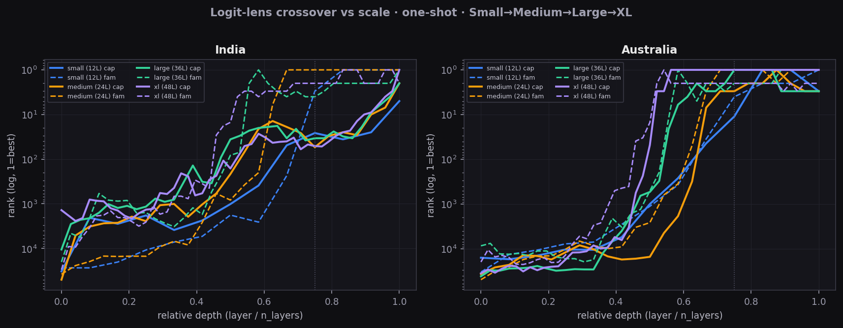
The mechanism is preserved, and engages earlier
| Country | Small | Medium | Large | XL |
|---|---|---|---|---|
| India | 0.75 | 0.625 | 0.556 | cleared |
| Switzerland | 0.75 | 0.458 | cleared | cleared |
| Australia | 1.00 | 0.917 | 0.889 | cleared |
| Canada | 1.00 | 0.958 | 0.889 | cleared |
The early-dominance crossover marches earlier in relative depth as the model grows — the larger model commits to the prior sooner, proportionally, before it has the capacity to overturn it. Then at XL the crossover disappears entirely.
Over-conditioning is capacity relative to task difficulty
The failure is not removed all at once but along a graded clearing threshold — harder cases (stronger frequency bias) require more capacity. What scale buys is not a weaker prior but enough capacity to override it once context is supplied. The inverted ICL gradient is not a quirk of one model size — it appears at GPT-2 Small and clears by GPT-2 XL for this task, and the natural unification is that over-prompting reflects model capacity relative to task difficulty. A 1.5B model exits the over-conditioning regime on capital-from-context; a frontier model exits that trivially and re-enters only on harder tasks — which is exactly where GPT-4o is observed to degrade.
X. The Over-Conditioning Framework
One in-context example teaches the task pattern, activating the retrieval circuit (L9H8, L8H11, L10H0). For most countries, this retrieves the correct capital — accuracy jumps to 79%.
Additional examples add more city names to the context. The retrieval circuit has no way to distinguish "example city" from "answer city." Each additional city name loads the prior heavier. The result is a degradation curve that looks like ICL failing but is mechanistically something more specific: the retrieval circuit is being asked to compete against its own prior.
The CFG parallel (speculative)
Classifier-free guidance in diffusion models (Ho & Salimans, 2022) shows a behaviorally similar tradeoff:
| Regime | Diffusion (CFG) | ICL (this work) |
|---|---|---|
| Conditioning too low | Ignores prompt → incoherent output | n=0: no cities |
| Optimal conditioning | Sharp, prompt-consistent output | n=1: 79% accuracy |
| Conditioning too high | Mode collapse → dominant prior modes | n=5: 55%, collapses to famous cities |
In diffusion models, too much guidance scale causes collapse toward whatever the unconditional prior finds most probable. The ICL gradient follows the same shape. Whether this is the same underlying phenomenon or merely analogous is an open question. The behavioral parallels are real; the mechanistic connection is not formally derived.
XI. Limitations
Scale. The detailed circuit analysis is from GPT-2 Small; specific head indices and effect sizes are properties of this model. The behavioral and logit-lens analysis extends across the GPT-2 family; full causal circuit analysis at scale is left to future work.
Sample size. The mechanistic analysis uses 5 error countries and 2 control countries.
Example order. The ICL examples always appeared in the same order. The Belgium→Barcelona error suggests order matters.
Activation patching limitations. The corrupted prompt (country replaced with "Dead") is one reasonable choice, not the uniquely correct one. Patching can miss distributed circuits and cancellation effects.
XII. Conclusion
One: one in-context example is optimal. Each additional example degrades accuracy monotonically, from 79% at one to 55% at five, driven by the model predicting famous cities with increasing confidence.
Two: the mechanism is a shared retrieval circuit that cannot distinguish factual associations from frequency associations. Attention heads L9H8 and L8H11 promote both the correct capital and the famous city for every error country tested. The winner is determined by the relative strength of associations in the training-data-derived weight matrix. More examples activate this circuit more strongly, which benefits the frequency prior disproportionately.
Three: the entropy-accuracy divergence is a practical warning. Monitoring entropy would miss this failure mode entirely.
Four: over-conditioning is capacity-relative. Persistent error count falls monotonically (5 → 4 → 3 → 0) across the GPT-2 family, reaching zero at 1.5B. The mechanism does not disappear with scale — it moves up the difficulty axis.
Next: Steering the Prior — what happens when we try to fix the failure by intervening directly in the residual stream.
Code: new_experiments/. Corpus analysis: exp_freq_analysis.py. Brazil probe: brazil_verify.py. Scale sweep data: scale_results/.